9. Background and Related Information
Last update: October 8, 2025 18:19 UTC (adf2ca217)
This section presents some background information and other related stuff that one may find interesting or entertaining.
9.1 Miscellaneous
9.1.1 What is Mills-speak?
9.1.2 How can I convert a date to NTP format?
9.1.3 How can I convert an NTP Timestamp to UNIX Time?
9.1.4 Where can I find more Information?
9.2 GPS
9.2.1 Selective Availability revisited
9.1 Miscellaneous
9.1.1 What is Mills-speak?
Most people using NTP know that it has been invented by Professor David L. Mills. So they frequently address him to solve their problems. Unfortunately they mostly don’t know about Mills-speak, the language used by the aforementioned person. To avoid some disappointment, I’ll give a small example of Mills-speak.
Example 9.1a: Mills-speak
Someone once had the misconception that the thing referred to as “nanokernel” was a kernel even smaller than a “microkernel”. Forwarding the problem to Professor David L. Mills, the answer was:
“A nanokernel is a species of korn. Korn is grown on Jupiter as a dietary supplement by the Nanos, a prehistoric people of predominantly aquatic descent. The ancient enemy of the Nanos are the Micros, who also grow a variety of korn. Their variety is closely related to the eggplant of today, although we know the eggplant is distantly related to chickens. In Micro mythology, chickens farm fields of eggplants that are specially grafted to korn and eventually evolve and emerge as hackers. Both Nanos and Micros prize hackers, which when planted in fields of chicken manure greatly vex the environmental authorities, since the confluence of the two peoples generally degenerate to clouds of messy, smelly swamp gas.”
Another example follows.
Note: I’m not sure what question this answer refers to, but it could be referring to the fact that some black box NTP servers exist that use Linux as operating system. If you can correct me, please do!
Ulrich,
Fancy that; when you pop the cover off the CPU chip, a little guy with pointy ears and a pitchfork snarls back at you. Like the time I popped the lid off a digital wristwatch and found a little Micky Mouse etched in the silicon.
Dave
Still another one dealing with specifications of clock errors:
Colin,
A little clarification. 12 PPM = 12 parts per million = 12 microseconds per second = 43 milliseconds per day = 0.602 seconds per fortnight. Most computer clocks have systematic frequency errors less than 100 PPM, but some considerably more. These errors are due to the manufacturing tolerance and each clock oscillator is different.
Computer clocks are like a cat who never remembers where it has been, only steps ahead in more or less random directions. The cat has a general idea in which direction leads to food, just not a precise idea of how to get there. Mathematically, this represents random walk frequency noise. The important fact about this is that predictions of future cat directions get worse more rapidly as future time recedes.
The “after one year” has to do with crystal aging characteristics. The cat gets old and starts steering more to one direction than the other. Really clever clock discipline algorithms attempt to learn the particular cat aging characteristic and compensate for it. Unless you are talking about oven controlled quartz or rubidium or cesium, this is not something we do with computer cats.
This brings up the notion of specifications “after one day”. Whoever said that doesn’t understand cats. The cat forgets just about everything after maybe an hour. Anything said after one day applies equally after one hour as the cat wanders. The really ugly bottom line is that, considering the cat’s memory, it doesn’t make sense to try to discipline the feline by averaging things over much more than a thousand seconds or so. Lots and lots of professional folks who should know better don’t understand this.
Most folks, including me, characterize each clock oscillator in terms of what is called Allan deviation. The bottom line is that most computer clocks can steer to something like 1 PPM relative to its intrinsic frequency error and without outside discipline as long as nothing violent temperature-wise is happening.
Dave
As David Craggs (and others) pointed out, the calculation is obviously wrong: 12 PPM correspond to 43 ms per hour, and not per day. Likewise an error of 0.602 s per fortnight corresponds to a frequency error of 0.49 PPM.
NTP uses seconds since 1900, while UNIX uses seconds since 1970. The following routine by Tom Van Baak will convert the times accordingly:
/*
 * Return Modified Julian Date given calendar year,
 * month (1-12), and day (1-31). See sci.astro FAQ.
 * - Valid for Gregorian dates from 17-Nov-1858.
 */

long
DateToMjd (int y, int m, int d)
{
    return
        367 * y
        - 7 * (y + (m + 9) / 12) / 4
        - 3 * ((y + (m - 9) / 7) / 100 + 1) / 4
        + 275 * m / 9
        + d
        + 1721028
        - 2400000;
}

/*
 * Calculate number of seconds since 1-Jan-1900.
 * - Ignores UTC leap seconds.
 */

__int64
SecondsSince1900 (int y, int m, int d)
{
    long Days;

    Days = DateToMjd(y, m, d) - DateToMjd(1900, 1, 1);
    return (__int64)Days * 86400;
}
9.1.3 How can I convert an NTP Timestamp to UNIX Time?
The following Perl code presented by Terje Mathisen (slightly improved by Ulrich Windl) will do the job:
# usage: perl n2u.pl timestamp
# timestamp is either decimal: [0-9]+.?[0-9]*
# or hex: (0x)?[0-9]+.?(0x)?[0-9]*

# Seconds between 1900-01-01 and 1970-01-01
my $NTP2UNIX = (70 * 365 + 17) * 86400;

my $timestamp = shift;
die "Usage perl n2u.pl timestamp (with or without decimals)\n"
    unless ($timestamp ne "");

my ($i, $f) = split(/\./, $timestamp, 2);
$f ||= 0;
if ($i =~ /^0x/) {
    $i = oct($i);
    $f = ($f =~ /^0x/) ? oct($f) / 2 ** 32 : "0.$f";
} else {
    $i = int($i);
    $f = $timestamp - $i;
}

my $t = $i - $NTP2UNIX;
while ($t < 0) {
    $t += 65536.0 * 65536.0;
}

my ($year, $mon, $day, $h, $m, $s) = (gmtime($t))[5, 4, 3, 2, 1, 0];
$s += $f;

printf("%d-%02d-%02d %02d:%02d:%06.3f\n",
       $year + 1900, $mon+1, $day, $h, $m, $s);
There are various sources of information about NTP. The following list is definitely not complete, but probably a good starting point:
- This NTP website has a lot of information about NTP and related topics.
- There is also the NTP Support Wiki.
- One of the oldest sources of useful information is the NTP questions mailing list. That list is visited by many beginners as well as a few experts, and occasionally even the father of NTP posted a note there.
- The page Time, with focus on NTP and Slovenia contains a good summary of time synchronization using NTP as well as valuable references. The author allowed inclusion of his material into this FAQ. I really appreciate that.
- Technical papers by Professor David L. Mills are available in the Reference Library.
- Various RFCs deal with NTP. While newer RFCs obsolete older ones, it might still be interesting to read the older ones.
Table 9.1a: Some RFCs related to NTP
- Never underestimate the usefulness of Internet Search Engines like Google. Take the time once to learn how to search efficiently, and benefit from that knowledge every time.
9.2 GPS
This section tries to give some information about GPS.
The Navstar Global Positioning System (GPS) was developed in the seventies by U.S. military forces to supply position and time information all over the world. The system (to be precise: the GPS Space Segment) consists of 28 satellites (also termed Space Vehicles) orbiting the earth in six groups with four satellites in each group, roughly 20000km above the surface (12 hour orbits). Current Kepler data can be found here. There is also some visualization software named WXtrack.
Each satellite has four atomic clocks (two Cesium, two Rubidium) for very high precision timing on board. (The very first and the latest satellites lack one Cesium clock.) Currently it is controlled by the United States Air Force Space Command, Second Space Wing, Satellite Control Squadron located at the Falcon Air Force Base in Colorado. The satellites are monitored and controlled from four additional terrestial stations: Hawaii, Ascension Island, Kwajalein, and Diego Garcia.
To maintain the specified accuracy, most of the satellites require daily updates of their data, but some of them can receive and store corrections for several days. Under normal conditions the attitude error of the satellites is within 0.5°, and the error on the surface is 16m. If no corrections are uploaded for 14 days, the positioning error on the surface will increase to 425m. After 180 days the error will be 10km. If a satellite operates without current correction data, it is in extended operation.
The carrier used by the satellites to broadcast is 1.57542GHz, and the basic information consists of a pseudo-random noise code of 1023 bits, sent within 1ms (clocked at 1.023MHz). The noise code is specific for each satellite, modulating the base carrier to produce a spread-spectrum signal. Transmission starts at the beginning of a new millisecond. This allows setting the receiver’s clock modulo to 1ms. The pseudo code can be used to lock the receiver within up to 10ns, depending on the noise of the signal. When using the carrier phase, the phase in the receiver could be correlated as close as 1ps.
Due to the military origin of GPS, the data is sent in a way that will not allow obvious decoding. For example, one bit stream is combined with a pseudo-random number sequence that spans seven days. Fortunately most of the secrets are explained today.
Basically the system works as follows:
-
All satellites are tightly synchronized clocks with well-defined orbits, defined in almanacs. Each satellite has an unique identification and frequency that allows them to send the same signal down to earth synchronously.
-
Depending on the position of the satellite and the location of a receiver on earth (and some other parameters like ionospheric delay), the signals from the satellites arrive at different times.
-
The receivers know the exact position of every satellite using the almanac or the ephemeris data of the satellite. Both are a collection of parameters that describe the orbit of a satellite in terms of time. Each satellite broadcasts the almanac and the ephemeris periodically together with the time.
-
Initially every receiver has to get a rough estimate of its position, the current time, and the almanac. This process takes about 15 minutes to complete, frequently referred to as cold boot. Initially the receiver just listens to any satellite to get the current time, the satellite’s ephemeris, and the almanac. The almanac enables the receiver to concentrate on satellites that are within view, while the ephemeris helps to compensate for the delay and other distortions of the time signal.
If the receiver has a battery-buffered clock and RAM to save time, position, and almanac, it can perform a warm boot. During that procedure the receiver computes the visibility of the satellites using the almanac, the time, and the last position of the receiver. This simplifies the procedure of tuning to the right satellites.
-
Using the signals from three satellites, the receiver can determine its position relative to these satellites (2D mode, without elevation), already giving a rather exact time. With four or more satellites being received, the elevation can be computed as well (3D mode).
If a stationary receiver knows its position, it can provide accurate timing information with just one satellite in view, assuming the position does not change. If more satellites are in view, the GPS receiver can better calculate time approximation using overdetermined timing mode (limited to the number of receiver channels).
-
Even if the main purpose of GPS is getting the exact position, it is necessary to get the correct time first. When receiving four satellites or more, it is possible to uniquely determine the exact position of the receiver (imagine the intersection of spheres with a satellite at each center).
-
Depending on the exact position of satellites and the receive conditions, the achievable accuracy may vary, independent from the distortion that is added to the public signals. As the needed correction data are not publically accessible, this feature is named Selective Availability (SA).
The system offers two classes of precision:
-
High precision (Precision Positioning Service, P-code) for military use only (16m both horizontal and vertical).
-
Rough resolution (Coarse Acquisition, C/A-code, Standard Positioning Service) for public use (100m horizontal, 165m vertical). This service may be shut down or distorted in time of a crisis (or maybe whenever the military forces like to do so).
The precision may be further degraded by Selective Availability (SA) which was implemented in 1991, and turned off on May 2, 2000 at 0400 UTC.
Although derived from UTC, as presented by the U.S. Naval Observatory master clock, the UTC(USNO MC), GPS time does not include leap seconds found in UTC, but the data stream provides the difference from UTC in seconds. At the time of writing the difference is 18s. While the difference between UTC and GPS time will change over time, there’s a fixed offset between TAI and GPS time (19 seconds).
The latest versions of the GPS Interface Control Documents (ICDs) and Interface Specifications (ISs) are available from
https://www.gps.gov/technical-documentation.
Example 9.2a: A Glance at the GPS Sky
At the time of writing I could see five out of nine visible satellites, the best candidates being 24, 5, 4, and 9. From Table 9.2a you can see that my window is in the east, and that I have a rather nice view out there. From these data, GPS receiver computed my position as 49° 11' 42" N, 12° 16' 12" E, 260m.
Table 9.2a: GPS Satellites
| Number |
Elevation |
Azimuth |
Distance |
Doppler Effect |
| 4 |
24° |
50° |
23357km |
-1.151kHz |
| 5 |
63° |
80° |
20737km |
-1.462kHz |
| 9 |
27° |
146° |
23212km |
-3.446kHz |
| 24 |
34° |
94° |
22594km |
+1.237kHz |
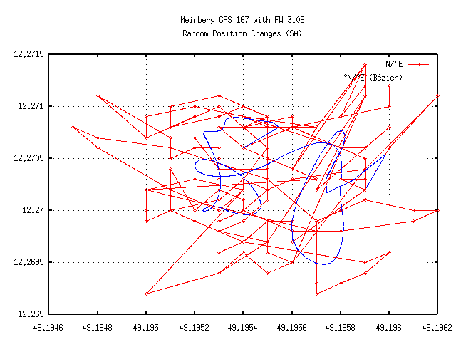
Example 9.2b: The Effects of Selective Availability
Most GPS receivers are unable to compensate for Selective Availability. As a virtually changing position causes time offsets (roughly 3ns per meter), it’s interesting what the effects of SA are. For my GPS167 from Meinberg I examined the gps_position(LLA) that the clock driver showed. The following graphic shows the changing position over time, including a smoothed path.
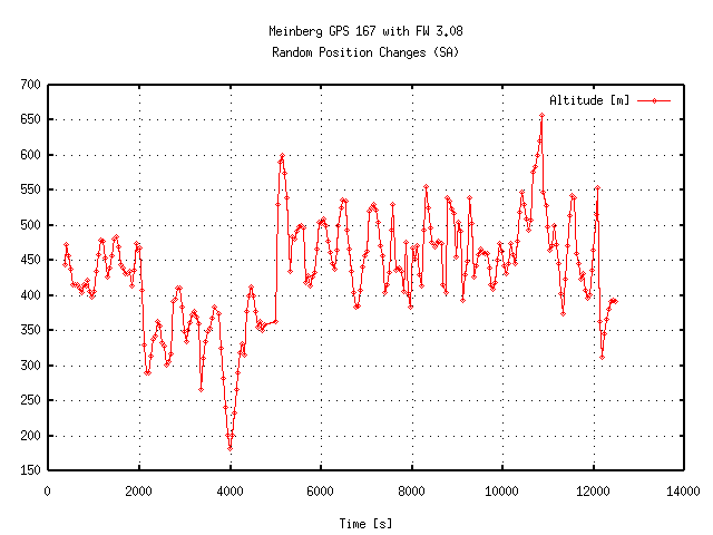
These position changes have a comparatively small effect on time accuracy, but if one considers the computed altitude, the huge changes can accumulate to a few hundred nanoseconds. The following graph shows the varying altitude over time.
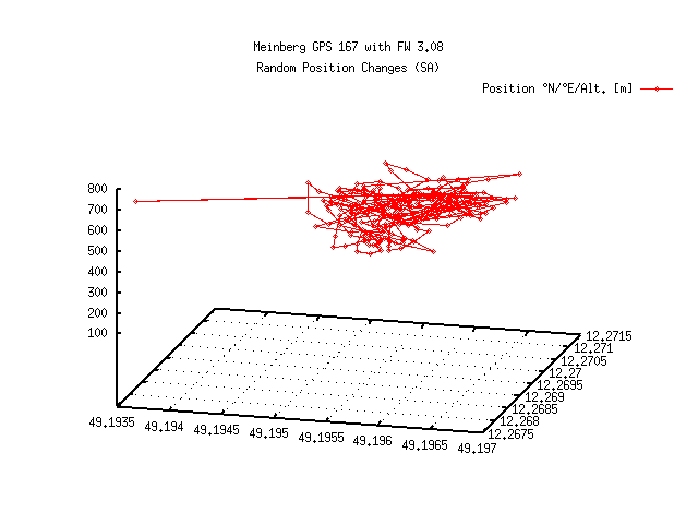
Finally, the following figure combines the three coordinates in space to give you an impression on how accurate GPS is:
9.2.1 Selective Availability revisited
On May 1st, 2000 there was an announcement about turning off Selective Availability (SA). The document titled President Clinton: Improving the Civilian Global Positioning System (GPS) quotes Bill Clinton: “The decision to discontinue Selective Availability is the latest measure in an ongoing effort to make GPS more responsive to civil and commercial users worldwide. –This increase in accuracy will allow new GPS applications to emerge and continue to enhance the lives of people around the world.”
However the algorithm that is used for SA is not explained, and it seems SA has just been replaced by more selective availability. “New technologies demonstrated by the military enable the U.S. to degrade the GPS signal on a regional basis. GPS users worldwide would not be affected by regional, security-motivated, GPS degradations, and businesses reliant on GPS could continue to operate at peak efficiency.” Pay attention to the wording (…) “could continue to operate (…)").